Excel Conditional Formatting Based On Reference Cell

How to format a row of cells based on the string value of a reference cell.

Note: These bits of code are mostly for my own reference, but if anyone else finds them useful all the better.

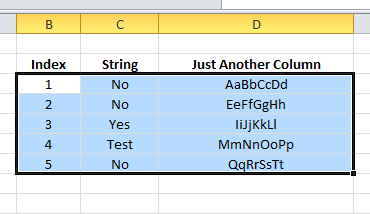
1. Select the range of cells to be conditionally formatted. Goofy things appear to happen depending on how you select. (i.e. where is the highlighted cell after selection). The image shows the highlighted cell in the upper left, achieved by selecting from upper left to lower right

.

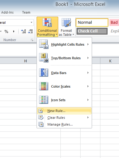
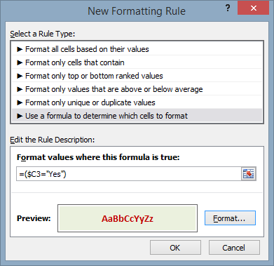
2. Choose: “Conditional Formatting” > “New Rule” > “Use a formula to determine which cells to format”

1. Enter the formula in the format: =(<REFERENCE CELL>=<TEXT STRING WITH QUOTES>). In the example this is

   . You use the “$” to control how the reference cell is translated across the selection.

4. Click through the OKs and you are done.